机器人的现代数学知识(Lie Groups)

参考：
paper: A micro Lie theory for state estimation in robotics
lib: manif
lib: sophus
book:《Modern Robotics Mechanics, Planning, and Control》Kevin M. Lynch, Frank C. Park (讲解视频) book:《机器人学的现代数学理论基础》丁希仑
videos: 南科大

1 基础知识

frame (physics) coordinate systems (mathematics)

自由向量（free vector）

• geometric quantity with length and direction

无坐标的（coordinate free）

• $p$ denotes a point in the physical space
• A point $p$ can be represented by a vector from frame origin to $p$
• ${}^Ap$ denotes the coordinates of point $p$ wrt frame $A$
• When left-superscript is not present, it means the physical vector itself or the coordinates of the vector for which the reference frame is clear from the context.

反对称矩阵（skew-symmetric） \(w=[w_1,w_2,w_3]^T\)

$[w]$ is called a skew-symmetric matrix representation of the vector $w$

有的也用 $\hat{w}$ 表示 skew-symmetric

$a \times b = [a]b$: cross product 本质上对后面这个vector进行了一个线性变换

旋转矩阵(Rotation Matrix) Frame: 3 coordinate vectors(unit length) $\hat{x}, \hat{y}, \hat{z}$ and an origin

• $\hat{x}, \hat{y}, \hat{z}$ mutually orthogonal
• $\hat{x} \times \hat{y} = \hat{z}$, right hand rule

Rotation matrix: specifies orientation of one frame relative to another

where, ${}^A\hat{x}_B$ 是$\hat{x}_B$在A frame下的coordinate

Properties:

根据后面李群的知识：\(R \in SO(3)\)

齐次变换矩阵

根据后面李群的知识：\(T \in SE(3)\)

欧式空间、非欧空间

• 欧式空间：距离、面积、体积等
• 非欧空间：黎曼几何、曲率等

角速度（angular velocity） \(w= \hat{w} \dot{\theta}\)

$\hat{w}$ 表示单位转轴（unit vector），$\dot{\theta}$表示角速度（scalar）

2 群

问题：为什么会引入群这个概念？ 回答：

看这个视频总结的

群是 一种集合 + 一种运算 的代数结构：记集合为$A$，运算为$\cdot$，当运算满足封闭性 Closure、结合率 Associativity、幺元 Identity element、逆 Inverse element四条性质，称$(A,\cdot)$为群

群的4个基本性质：封闭性、结合律、幺元律、可逆性

交换群(commutative group)、阿贝尔群(Abelian group)

• 旋转矩阵集合 + 矩阵乘法构成群 $\to$ 三维特殊正交群/旋转矩阵群$SO(3)$
• 变换矩阵集合 + 矩阵乘法构成群 $\to$ 三维特殊欧式群/变换矩阵群$SE(3)$
• 常见的其他群
  • 一般线形群$GL(n,\mathbb{R})$: $n\times n$的可逆（非奇异）实矩阵（二元运算：矩阵乘法），也可以记作: $GL(n)$
  • 特殊正交群$SO(n)$: $n\times n$的单位正交实数矩阵（二元运算：矩阵乘法），$SO(2)$、$SO(3)$是两个比较重要的子群。
  • 特殊欧式群$SE(n)$: 三维特殊正交群$SO(3)$和向量空间$\mathbb{R}^3$的半直积为特殊欧式群$SE(3)$: $SE(3)=SE(3)\otimes \mathbb{R}^3$，$SE(3)$也是特殊欧式群的一个子群。

3 李群

3.1 李群

李群：群的4个基本性质+3个特殊条件（可微流形、群的积是可微分的映射、群的逆也是可微分的映射）

一般意义的李群指的的乘法，不是加法。即矩阵李群。

典型例子：

• $n$维向量空间 $\mathbb{R}^n$
• 单模复数群 $z = \cos\theta + i\sin\theta$
• 一般线性群 $GL(n,\mathbb{R})$ - $n\times n$ 非奇异实数矩阵
• 正交群 $O(3)$ - $n\times n$ 正交实数矩阵
• 特殊正交群 $SO(n)$ - $n\times n$ 单位正交实数矩阵
• 三维旋转群 $SO(3)$
• 三维特殊欧式群 $SE(3)$
• 幺模群
• 特殊幺模群

3.1 李子群

组合运算 composition

• 直积direct product

• 半直积semi-direct product

交运算 intersection

• 李子群的交集还是李子群

商运算 quotient

4 李代数

4.1 李代数

李代数对应李群的正切空间，它描述了李群局部的导数。

李群：大写，例如$SE(3)$，$SO(3)$ 李代数：小写，例如$se(3)$，$so(3)$

• $SE(3)$的李代数是$se(3)$
• $SO(3)$的李代数是$so(3)$

李群表示刚体运动、李代数表示刚体运动速度，李群和李代数是指数映射关系。

4.2 指数映射

4.3 伴随表达

5 李括号

6 总结

6.1 SE(3)、SO(3)、se(3)、so(3)

1、$3 \times 3$ 旋转矩阵组成的集合称为特殊正交群（special orthogonal group）$SO(3)$

• 特殊正交群$SO(3)$称为旋转矩阵群
• 特殊正交群$SO(2)$是所有$2 \times 2$实数矩阵的集合，二维的

2、特殊欧氏群（special Euclidean group）$SE(3) $，称为刚体运动群、齐次变换矩阵（homogeneous transformation matrice）群

刚体的位形空间可以表示为$SO(3)$与$\mathbb{R}^3$的乘积空间（半直积）记作$SE(3)$

3、大写是李群、小写是李代数；他们之间是指数映射的关系；如下面两个exp的关系；

针对刚体运动，无论齐次坐标表达，还是伴随表达，都是具有指数映射关系$A=e^{\theta S}$;$Ad(g)=e^{\theta ad(j)}$

4、 所有$3 \times 3$反对称矩阵的集合称为$so(3)$，$so(3)$是三维旋转群的李代数 For any unit vector $[\hat w] \in so(3)$ and any $\theta \in \mathbb{R}$ \(e^{[\hat w]\theta} \in SO(3)\)

For any $R \in SO(3)$,there exists $[\hat w] \in \mathbb{R^3}$ with $||\hat w||=1$ and $\theta \in \mathbb R$ such that \(R=e^{[\hat w]\theta}\)

The vector $\hat w\theta \in \mathbb{R^3}$ is called the exponential coordinate for $R$

import packages.Python.modern_robotics.core as mr
import numpy as np
from scipy.linalg import expm, logm

R = np.array([[0, -1, 0], [1, 0, 0], [0, 0, 1]])

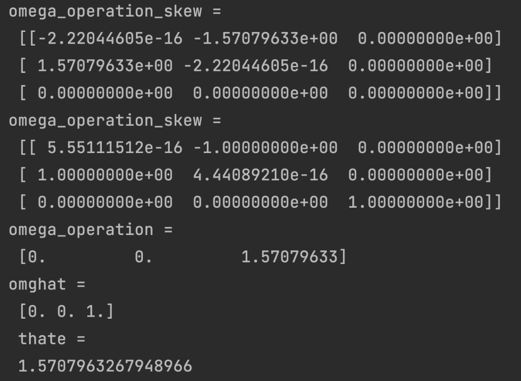
omega_operation_skew = logm(R)
print('omega_operation_skew = \n', omega_operation_skew)
R_test = expm(omega_operation_skew)
print('omega_operation_skew = \n', R_test)

omega_operation = mr.so3ToVec(omega_operation_skew)
print('omega_operation = \n', omega_operation)
omghat, thate = mr.AxisAng3(omega_operation)
print('omghat = \n', omghat, '\n', 'thate = \n', thate)

结果如下所示：

Rodrigues’Formula: Given any unit $[\hat w] \in so(3)$,we have \(e^{[\hat{w}\theta]} = I + [\hat{w}]sin(\theta)+ [\hat{w}]^2(1-cos(\theta))\)

证明：将指数按照幂级数展开，再结合$sin(\theta)$和$cos(\theta)$的展开，化简。

刚体运动的指数坐标

矩阵指数$e^{\mathcal{S} \theta}$

import packages.Python.modern_robotics.core as mr
import numpy as np
from scipy.linalg import expm, logm
np.set_printoptions(suppress=True)

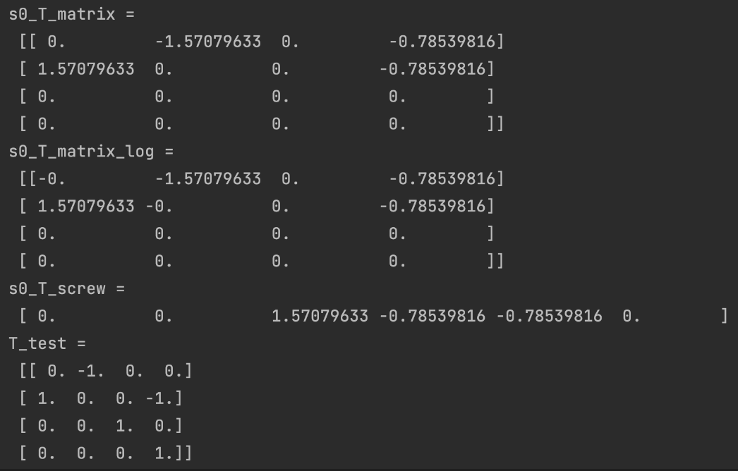
T = np.array([[0, -1, 0, 0], [1, 0, 0, -1], [0, 0, 1, 0], [0, 0, 0, 1]])

s0_T_matrix = mr.MatrixLog6(T)
print('s0_T_matrix = \n', s0_T_matrix)
s0_T_matrix_log = logm(T)
print('s0_T_matrix_log = \n', s0_T_matrix_log)
s0_T_screw = mr.se3ToVec(s0_T_matrix)  # 得到Twist
print('s0_T_screw = \n', s0_T_screw)
T_test = expm(s0_T_matrix)
print('T_test = \n', T_test)

结果如下：

6.2 不同表达、不同运算

不同表达对应不同的运算，各有各的好处。

伴随表达也具有指数映射的关系$Ad(j)=e^{\theta ad(j)}$

• 3×3表达的旋转运动的李群$T$和其对应的李代数

• 齐次坐标表达的刚体运动的李群$T$和其对应的李代数

\[T^{-1} = \begin{bmatrix} R^T & -R^Tp \\ 0 & 1 \end{bmatrix}\]

• 伴随表达（adjoint rspresentation）的刚体运动的李群$Ad_T$和对应的李代数

$Ad_T$ 也可以表示成 $Ad(g)$

7、旋量理论与机器人运动学

所有的刚体运动都可以用螺旋运动表示。

旋量是一条有节距的直线；当节距=0，旋量$\to$线矢量。

7.1、齐次坐标与线矢量

点的齐次表示

面的齐次表示

线的齐次表示

Plucker坐标

线几何（线矢量）：

线矢量（line vector）：依附在空间某一直线上的向量（p29，戴建生）

$s$称为原部矢量，$s_0$称为偶部矢量

线矢量，点乘没有意义；不过可以计算代数和、互易积（reciprocal product）

7.2、旋量、螺旋运动

• 如果是4×4表达，利用共轭运算conjunction，可以进行刚体变换：$T = T_2T_1T_2^{-1}$
• 如果是伴随表达，即4×4，共轭运算和伴随表达是等价的，即：

Twist / Spatial vector（运动旋量）、screw motion（螺旋运动）

运动旋量写成矩阵的形式 \([\mathcal{V}_b] = \begin{bmatrix} [w_b] & v_b \\ 0 & 0 \end{bmatrix} \in se(3)\)

运动旋量 $\mathcal{V}$ 可以写成螺旋轴（screw axis）$\mathcal{S}$与绕该轴转动的速度的组合形式

1、Consider “unit velocity” $\mathcal{V} = \mathcal{S}$
2、if not unit speed $\mathcal{V} = \mathcal{S}\dot \theta$
3、$\mathcal{V} = ScrewToTwist(\hat w,h,q,\dot \theta)=ScrewToTwist(\hat w,h,q,\dot \theta=1)\dot \theta$

screw motion \(\mathcal{V} = [w;v]=[\hat{s}\dot{\theta};-\hat{s}\dot{\theta}\times q+h\hat{s}\dot{\theta}]=[-w \times q+hw]\)

7.3、Forward Kinematics

参考：

calculation of the configuration（pose） $T=(R,p)$ of the end-effector frame from joint variables $\theta =(\theta_1,…,\theta_n)$

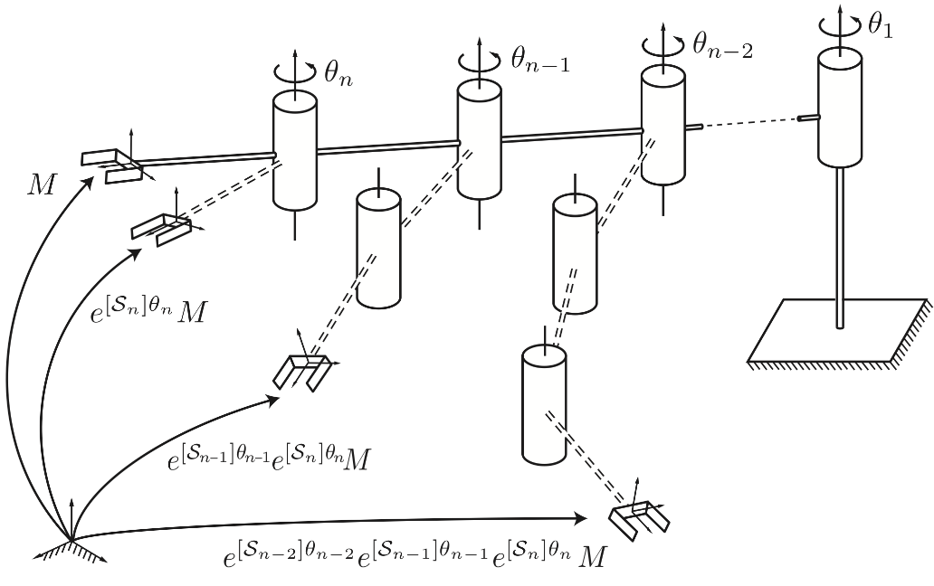
PoE（Product of Exponential）Formula \(T_{sb}(\theta_1,...,\theta_n)=e^{[^{0}\mathcal{S}_1]\theta_1} e^{[^{0}\mathcal{S}_2]\theta_2} ... e^{[^{0}\mathcal{S}_n]\theta_n}M\)

1、所有$\theta = 0$,计算初始$M$ 2、从后往前，转动最后一个关节，其余关节为0 3、继续转动倒数第二关节，其余关节为0 4、。。。 5、按照screw motion计算，在计算PoE公式

步骤：

1. 建立坐标系（基坐标系${S}$，工具坐标系${T}$），只需要这两个坐标系，其他关节确定关节轴线或者移动方向即可。
2. 计算$\theta_1 = …=\theta_n=0$时的初始位形，基坐标系与工具坐标系的$M$的变换${}_T^S{g(0)}$
3. 计算$w_i$，
4. 关节轴线上的一个点，所以那个$r_i$并不固定，但是不影响计算结果。
5. 计算单位运动旋量$\xi_i=[w_i,r_i\times w_i]^T$（转动副），$\xi_i=[0, v_i]^T$（移动副）
6. 根据公式：$e^{\theta \hat\xi} = \begin{bmatrix} e^{\theta \hat w} & ({I}-e^{\theta \hat w})(w \times v) + \theta ww^Tv
   0 & 1 \end{bmatrix}$,$w \neq 0$
7. ${}_T^S{g(\theta)}=e^{\theta_1 \hat\xi_1} e^{\theta_2 \hat\xi_2} \dots e^{\theta_i \hat\xi_i} \dots e^{\theta_n \hat\xi_n} {}_T^S{g(0)}$

7.4、练习题

2自由度机器人(RR)

• P53

平面3自由度机器人(RRR)

• P55

空间3自由度机器人(RRR)

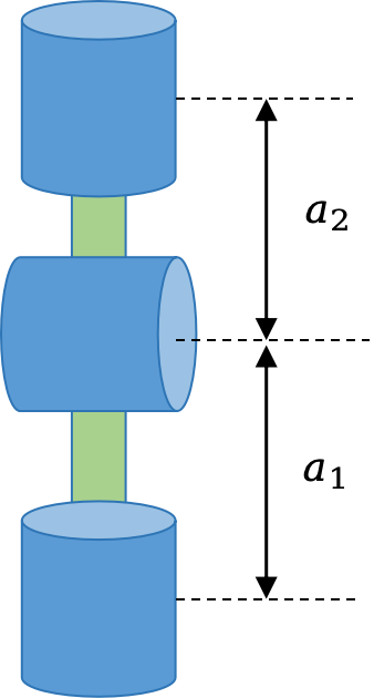
解

1. 建立如下图所示的坐标系
2. SCARA机器人(RRRP)

• P56

6自由度机器人(RRRRRR)

8、Inverse Kinematics

解析解的几种方法

9、Velocity Kinematics

deriving the Jacobian matrix:linearized map from the joint velocities $\dot \theta$ to the spatial velocity $\mathcal{V}$ of the end-effector

1、（重点） 空间雅可比（space Jacobian）,$J_s(\theta)$，简单理解为基于基坐标系的，或张巍老师讲的情况。 公式如下： \(J_s(\theta)=\)

2、物体雅可比（body Jacobian），$J_b(\theta)$，末端（物体）坐标形式下的雅可比矩阵。

10、Dynamics

11、旋量系、互异旋量系、运动旋量系、约束旋量系、等效运动副旋量系。。。

这部分内容偏机构学中的分析方法。